
This page summarizes relevant concepts and statistical techniques learned in A508 from the book Modern Statistical Methods for Astronomy. The focus is more on restating the ideas behind different techniques in a way that makes sense to me (specifically those that were mentioned more than just in passing during class), than just regurgitating information from the book.
The meaning and goals of statistics are debated, but it's basically a tool for interpreting data. There is a lot of human influence when using statistics and how it applies to data, so everything will be up to the scientist's interpretation, to at least some degree.
Astronomers tend to believe that the underlying physical processes can be uncovered by analysis of observations. However, there are many challenges and options that one can use, and it is far too easy to reach different conclusions based on different interpretations and statistical analyses of the same data.
Interesting, but not terribly relevant to the goal of this website.
It is usually impossible to measure everything about every member of a population, and those measurements that are taken are not infinitely accurate or precise. There is always some limit to our knowledge, represented by uncertainty.
Most of the terms defined here are in common usage and are pretty obvious, but it can be helpful to define them in a specific way.
Experiment - Any action whose results are not known with complete certainty before the action occurs.
Outcome space or sample space - The collection of all possible outcomes of the experiment.
Event - A subset of the sample space. Not necessarily a single outcome. In the sample space of all stars within 50 pc, one event could be all stars with an apparent magnitude < 10, while another event tells whether a star is in a binary system.
The simplest probability is when all outcomes are equally likely, so the probability of an event occurring is simply the number of favorable outcomes divided by the total number of possible outcomes.
For simple problems, sometimes you can just use logic to assign probabilities if the outcomes can be constructed out of outcomes from a simple experiment like the definition italicized above.
Discrete sample space - any finite or countably infinite sample space.
In general, the probability of an event occurring is equal to the sum of individual outcomes that are favorable to the event.
Probability space - Described by three objects: Ω, F, and P. Ω is the sample space, F is the class of events (a collection of events from the sample space), and P is a function that assigns probabilities to each event in F.
Axiom 1: The probability of any event must be between 0 and 1.
Axiom 2: The sum of all probabilities must equal 1.
Axiom 3: The probability of at least one of a set of mutually exclusive events occurring is the sum of their individual probabilities. This is known as countable additivity.
The probability of the complement of an event is simply 1 minus the probability of the event.
The probability of the union of two events is equal to the sum of the individual event probabilities minus the probability of the intersection. This can be extended to the inclusion-exclusion formula.
Necessary for understanding Bayesian statistics. The probabilities of events can sometimes depend on previous knowledge about the system. Defined in words, the probability of A given B equals the probability of the intersection of A and B divided by the probability of B. An extension of this definition is the
Multiplication rule -
This is a very important concept for astronomy, since there is almost always at least some previous knowledge available for any given object.
The multiplication rule also leads to the
Law of total probability -

where Bi is a partition of the sample space. All of this finally leads to
Theorem 2.1 (Bayes' Theorem):
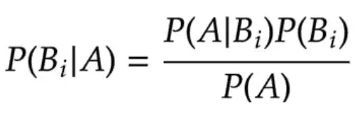
where P(A) is defined by the law of total probability.
If P(A|B) = P(A), then A and B are independent. In other words, the probability of independent events occurring is the product of the individual probabilities.
Random variables - functions on the sample space. For example, the number of heads that you get when flipping a coin four times is a random variable on the sample space of all sets of four coin flips.
Cumulative distribution function - The probability as a function of x that the value of a random variable is less than or equal to x.
Probability density function - The integral of the pdf over a range of values equals the probability of the random variable having a value within that range.
The idea of a random variable can be extended to a random vector of variables. Grouping variables this way allows you to study the relationships between variables instead of just each variable individually.
Marginal distribution - The 1-D distributions of individual variables from the random vector. They act like a regular CDF.
Just like independent events, independent RVs have their joint distribution equal to the product of the marginal distributions.
Moments - Mathematically, the kth moment of f(x) is the integral over the sample space of f(x) to the kth power times the pdf.
Central Moments - Moments where the RV first has the expectation subtracted out
Mean/First moment - also called the expected value or expectation value
Variance - Second moment minus first moment squared, describes the spread of a function.
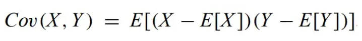
Covariance - measures the relationships between scatter in two RVs. Independent RVs have Cov = 0.
Skewness - Third central moment. Describes which direction the RV leans
Homoscedastic - If all variables have the same variance. The opposite is heteroscedastic. For independent variables, the sample mean is the sum of all the RVs divided by the number of RVs, and the variance is the homoscedastic variance divided by the number of RVs.
Standard deviation - the square root of the variance
Standardized form of a variable - The variable minus the mean and divided by the standard deviation. This removes any units associated with the variable.
Independent and identically distributed - i.i.d. for short. The assumption that data are all generated from the same population or underlying distribution. For example, if you repeat the same experiment multiple times. Many methods require i.i.d. variables, so be careful.
Quantile function - The inverse of the CDF. It is the measurement of the value of the RV at which a specific fraction of the CDF has passed. For example, the 95% quantile tells what the value of the random variable is when the CDF reaches 0.95.
Bernoulli distribution - An experiment that can result in only two outcomes, where the probability of one is p and the other is 1-p.
Binomial distribution - A Bernoulli trial is repeated n times independently. The binomial distribution describes the probability of a given number of successes. X ~ Bin(n,p). Mean = np. Variance = np(1-p)

Poisson distribution - A good approximation for binomial probabilities when pn is small, n is large, and λ=npn is a reasonable value. Describes many physical phenomena where counting statistics are important (photons hitting a detector, nuclear decay, etc.). Mean = Variance = λ

Negative binomial distribution - Known as the geometric distribution when r = 1. Mean = r/p, Variance = qr/p2.
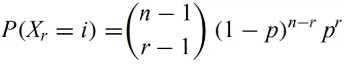
for n=r, r+1, . . . ,
Uniform distribution - constant between bounds a and b. f = 1/(b-a), a < x < b. Mean = (a+b)/2, Variance = (1/12)(b-a)2.
Exponential distribution - F(x) = 1 - e-λx, f(x) = λe-λx, x ≥ 0. Mean = 1/λ, Variance = 1/λ2. This distribution displays
Memorylessness - The property that the probability that the RV is greater than t + s given that it is greater than s equals the probability that the RV is greater than t (for positive s, t). This property is necessary for being able to model waiting times for Poisson processes.
Normal/Gaussian distribution - The bell curve, the limit of the central limit theorem, describes natural processes that depend on many uncorrelated variables. RV with this pdf is a normal RV. Mean μ, Variance = σ2

Lognormal distribution -


It is fairly simple to construct distributions with discontinuities. When this is the case, to calculate moments, you integrate xk with the CDF as the variable of integration using the Riemann-Steiljes integral.
Law of large numbers - for a sequence of i.i.d. variables, the sample mean will approach the expectation value (the population mean) as n goes to infinity.
Central limit theorem - for a sequence of i.i.d. variables, mean μ and variance σ2, then the probability approaches normal (known as asymptotic normality).

There is a lot of good example code in this section that shows you how to graph different distributions. No use repeating it here, since there's nothing to summarize. Just open the book if a specific example is needed.
When trying to learn about the underlying population, it is often possible to measure the properties of only a small sample of the full population of objects (often including bias). The inferences made are often based on a
Statistic - a function of random variables (mean, median, mode, standard deviation, etc. though they can, of course, become very complicated)
Inference is done basically any time a conclusion is drawn from astronomical data. Most of the rest of the book is based on different inference techniques. This chapter gives the foundations.
Statistical inference - the very broad category of methods to draw conclusions about underlying populations from observed samples (including intrinsic uncertainties). It can be used for estimation or to test hypotheses. It can be parametric (requiring assumptions about the underlying structure of the population, like linear regression), nonparametric (don't assume model structure), or semi-parametric (combine aspects of both, e.g., local regression).
Point estimation - The method of estimating the model parameters based on observations when the shape of the pdf of the underlying population is known (finding the mean and standard deviation of points drawn from a normal distribution, for example).
Maximum likelihood estimation - The likelihood is the hypothesized probability distribution that past events were drawn from. It differs from probability, since probability relates to future unknown events, while likelihood is an unknown distribution from known past events. MLE entails taking the maximum of the likelihood as the estimator for the statistic.
Confidence intervals - An x% confidence interval is likely to contain the estimated parameter with a probability of x%.
Resampling methods - point estimation methods are often inherently variable. This is necessary if one wants to determine confidence intervals, for example. Sometimes the variance is not possible to express easily, or at all. Resampling methods construct hypothetical populations from existing observations and then examine all of them simultaneously to determine intrinsic variations. Bootstrapping is one of the most common and powerful examples of these techniques.
Testing hypotheses - instead of estimating parameters, the goal is to test if data are consistent with a hypothesis. Null hypothesis (the claim that the studied effect does not exist or that there is no relationship between datasets or variables) and alternative hypothesis. The result is either reject or not reject the null hypothesis, which is not the same as saying the null hypothesis is correct. These types of tests can lead to false positives and false negatives, where the null hypothesis is wrongly rejected and wrongly failed to be rejected, respectively.
Bayesian inference - observational evidence is used to infer or update inferences. As more measurements are taken, the belief in any given model is likely to change. Encapsulated in the prior, the distribution that represents, in functional form, all previous knowledge about the problem.
Model misspecification - Care must be taken that the chosen model is a good fit for the chosen population or physical process.
Model validation - test of goodness-of-fit
Multiple ways to estimate best-fit parameters, including method of moments, least squares, and MLE. The correct choice will depend on the specific problem, but there are a lot of situations where it is possible to find the best-fit using techniques that are simultaneously unbiased, have minimum variance, and have maximum likelihood.
The point estimator of the true parameters is usually represented by theta hat and is a function of the random variables being explored. The estimator is calculated from a particular sample drawn from the population being estimated.
However, it is not always possible to optimize all the important properties of the estimator. Some of the important criteria of a point estimator are:
Unbiasedness - The bias of an estimator is the difference between the mean of an estimated parameter and its true value. This is an intrinsic offset in the estimator, not the error of one representation of the estimator from a particular dataset. Unbiased estimators have 0 bias, while asymptotically unbiased estimators have their bias approach zero as the number of data points goes to infinity.
Mean square error - The sum of the variance and the square of the bias. It is the expectation value of the estimator minus the true value, quantity squared. Used in the evaluation of estimated parameters.
Minimum variance unbiased estimator - a term for the estimator with the lowest variance in a collection of unbiased estimators. It is usually considered the most desirable.
Consistency - The trait of an estimator that approaches the true parameter as the sample size increases.
Asymptotic normality - when an ensemble of consistent estimators approaches a Gaussian distribution around the true value with a variance that decreases as 1/n.
Many probability distributions and models only depend on a few parameters. There are many techniques that one can use to obtain estimates of these parameters. The most common are the method of moments, least squares, and maximum likelihood estimation. For a Gaussian, for example, the mean and variance are estimated by the sample mean and sample variance, respectively.
Method of moments - Moments describe basic parameters of a distribution (central location, width, asymmetries). The kth sample moment is basically a discrete version of the kth moment. You sum up each sample value to the kth power and divide by the sample size. Any parameter that can be expressed as a simple function of the moments can be estimated in this way.
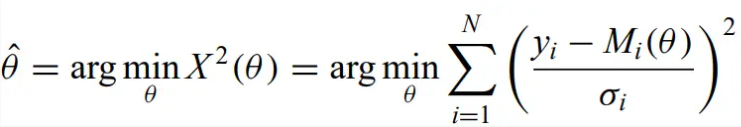
Method of least squares - A significant application of least squares is in regression (Section 7.3). The least-squares estimator of a parameter is obtained by minimizing the sum of the squares of the differences between the data and the population parameter being estimated. Weighted least squares is similar, but used for data with heteroscedastic errors. You instead minimize the weighted sum of squares, weighted by some known linear combination of parameters. This is related to Minimum χ2 regression.
Maximum likelihood method - Focuses on methods that give the most probable outcome for an estimator. The likelihood is the pdf viewed as a function of the data given model parameters with specific values. f(_;θ) is the pdf with parameter θ. Therefore, the likelihood and loglikelihood are given by:
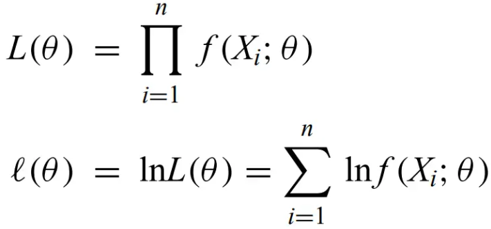
where Xi are i.i.d. random variables, and you replace X with x for observed data. loglikelihood is usually computationally easier to calculate. The MLE estimator is usually unbiased, but if it isn't, this can usually be fixed by multiplying the estimator by a constant. For “nice” functions g of the parameter, the MLE of g is the MLE of the estimator. Many common situations have the MLE estimators as asymptotically normal (this is helpful for calculating confidence intervals).
Coverage probability - The probability that the true parameter is within the x% confidence interval is at least x%. For a 95% confidence interval, if the experiment were repeated 100 times, an average of 95 intervals would contain the true parameter value.
MLE confidence intervals depend on the variance and sample size. The 100(1-a)% confidence interval for the mean is:

where z and t are defined such that P(Z > z) = P(Tm > t(m)) = a, where Z is the standard normal and Tm is a t-distribution with m degrees of freedom.
Other confidence interval calculations can quickly get even more complicated, but thankfully, statistics software is good at calculating them.
Two-sided and One-sided - Two-sided confidence limits are calculated when the question permits higher and lower values. One-sided is asymmetrical.
Any numerical optimization method can be used to maximize likelihoods. The simplest analytical model is to simply set the derivative of the likelihood to 0 with respect to each parameter. This gives a system of p equations in p unknowns that can be solved with algebra.
There have been computational methods with varying degrees of effectiveness, but one of the most influential is the
EM algorithm - considers mapping a set of datasets to an unknown complete set. The algorithm starts with initial values of the model parameters. The algorithm is iterative and has two steps: the expectation step calculates the likelihood for the current values of the parameter, and the maximization step updates the missing data values, assuring that likelihood with respect to the current model is maximized. This new dataset replaces the original, and the algorithm is repeated until convergence. This is useful since each step guarantees an increase in the likelihood from the previous iteration.
Two competing statements are determined for a given experiment. The null and alternative hypotheses. It is impossible to simultaneously minimize false positives and negatives, so the scientist must decide what is more important for the specific question. Most commonly, let false negatives be uncontrolled, and keep false positives down to the 5% confidence level.
Power - the probability of correctly rejecting the null hypothesis (i.e. when the alternative hypothesis is true) = 1 - false negative rate. Often want to look for the
Uniformly most powerful - describes the test statistic that gives the highest power for all parameters at a chosen significance level.
Statistically significant - the result of a test that is unlikely to have occurred by chance. Significant at the x level if you have 100(1-x)% confidence. Quantified also by the
p-value - the probability of getting a value as extreme as the test statistic, assuming the null hypothesis is true.
The null hypothesis can never be accepted; it can only (fail to) be rejected at a given confidence level. If many hypothesis tests are conducted on the same dataset (searching every pixel in an image for faint sources), significance levels must change. This is because there then must be a balance between false positives and sensitivity.
False detection rate - A new procedure for combining multiple hypothesis tests that can control false positives.


Critical regions (rejection regions) - If a statistic falls in the critical region, the null hypothesis should be rejected.
In the above tables, X bar is the sample mean of n i.i.d. random variables, and Y bar is the sample mean of m i.i.d. random variables from a population independent of x. y are observations from a binomial distribution with population portion p with n trials. If n and m are small, then different critical regions will have different definitions.
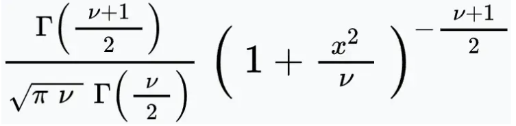
The t distribution - with v degrees of freedom. It is the sampling distribution for random samples from normal populations. If x bar and s2 are the mean and variance of a random sample of size n from a normal population, then (xbar - mu)/(s/sqrt(n)) has the t distribution with n-1 degrees of freedom.
Finding the distribution of any given statistic is often difficult in general. However, this limitation can be somewhat overcome with
Resampling methods - statistical methods that involve building synthetic populations from limited observations that can all be analyzed in the same way to see how statistics depend on random variations in the observations. Resampling methods do well to preserve the true distributions in the underlying real population, including things like truncation and censoring.
Half-sample method - randomly choose half the data points, calculate the statistic, and repeat. Estimation of the statistic can then be based on a histogram of the resampled statistics. Also called interpenetrating samples. One very popular variant of this is the
Jackknife method - For a dataset with n points, calculate n datasets ("jackknife samples") with n-1 points, each omitting a different point, then calculate the statistic for each sample. Helps with detecting variation with n (bias), as in general, we want n = infinity. Can fix bias of order 1/n, but not greater.
Bootstrap - Resampling with replacement. Create a large number of datasets, each with n points randomly drawn from the original data. This means that the simulated datasets will each miss some points and also have multiple copies of the same data point. In that way, it is a Monte Carlo method to simulate from existing data without any assumption of the underlying population (i.e., it is nonparametric). Useful for generating confidence intervals, as well.
There are a lot of situations where the “best fit” of a particular model to data is required. The overall procedure for doing so is:
The choice of model is outside the scope of the book and depends on the situation, but one should normally choose the simplest model that is consistent with the data.
Nested/nonnested models - nested models refer to the case where the simpler model is a subset of the more elaborate model(s) in question. These are easier to compare with one another.
Reduced χ2 statistic - To calculate, the model is compared to binned data and best-fit parameters are obtained by weighted least squares, and the weights are obtained from the dataset (like the standard deviation equaling the square root of the number of data points in the bin) or ancillary measurements (e.g. noise level in background of a CCD image).
Doing the above gets you the minimum χ2 parameters. Goodness of fit is chosen to be when χ2v is minimized, where v is the number of degrees of freedom.
There are three main categories of nonparametric hypothesis tests: those based on the KS, Cramer-von Mises, and AD statistics, and they are used to compare empirical distributions of univariate data to the hypothesized distribution function of the model. These are described in more detail in Section 5.3. It is important to state, however, that there is a distinction between the KS statistic and the KS test. Also, the pre-tabulated probabilities are only valid for models where all the parameters are estimated independently, which is uncommon in astronomy. This problem can be alleviated with bootstrapping.
Parametric bootstrap - simulated datasets are obtained from the best-fit model. Using this to get 90 to 99% critical values replaces the standard probability tabulation of the KS test.
Likelihood-based methods for model selection use hypothesis testing based on maximum likelihood estimators. Below are some examples:
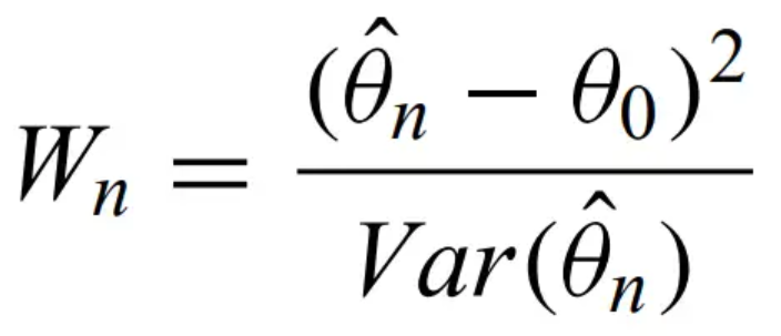
Wald test - provides a test for the null hypothesis that the value of the parameter equals theta naught. It represents the standardized distance between theta naught and the MLE theta hat.
Likelihood ratio test - use the ratio of the likelihoods for theta hat and theta naught.
Score test - uses this statistic.
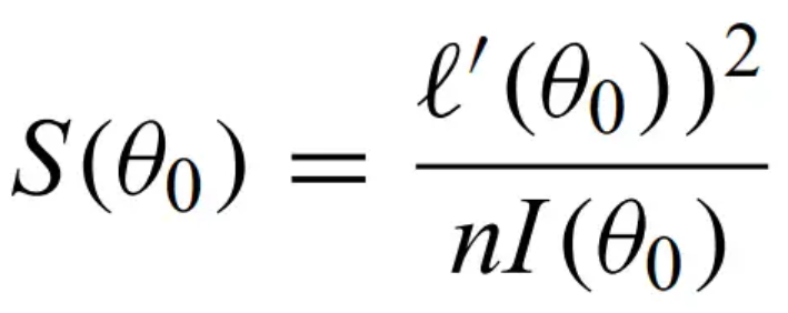
where l' is the derivative of the loglikelihood, and I is Fisher's information:
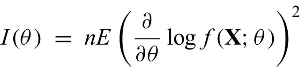
where X is a random variable and theta is a parameter.
Sometimes it is better to take an alternative approach with
Penalized likelihoods - when using nested models, the largest likelihood in the nested model is always the more complicated model because it has more parameters. So, you can apply a penalty to compensate for this difference.
Akaike information criterion - defined for model j as
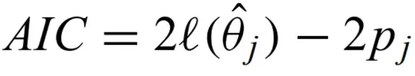
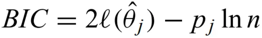
where p is the number of parameters in the jth model. The first term is goodness-of-fit, and the 2p is the penalty term. This criterion finds the model that maximizes the AIC. Another common criterion is the
Bayesian information criterion - where the penalty comes from the parameters and the number of data points
Posterior probability - the conditional probability of the model given the data. This is the result of the calculation.
Likelihood function - The conditional probability of the data given the model. The assumed distribution the data are drawn from.
Prior information - The marginal probability of the model. There is no information from the data, but this is where prior information about the problem is included.
The posterior of a chosen set of models given the observable is equal to the product of the likelihood of the data for those models and the prior probability on the models (normalized).
Bayesian inference - applying the steps above (Baye's theorem) to assess the degree to which a dataset is consistent with a hypothesis.
Bayesian inference works best when there is prior knowledge to get a realistic prior. Where MLE gives the maximum of the likelihood, Bayesian first weights this likelihood by the prior. Some useful prior distributions include:
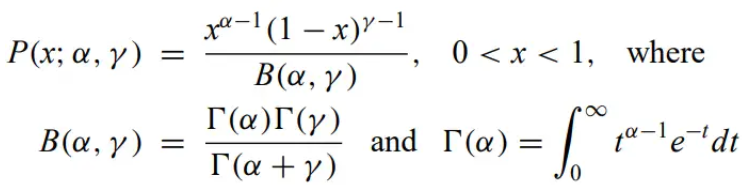
beta distribution - flexible choice for a prior
Maximum a posterior/highest posterior density estimate - MLE of the posterior.
Normal mixture model - unknown number of normal components
This chapter focuses on a few pdfs that are useful to astronomy. For any information not in the table below, look to Wikipedia since these are all common distributions.

As described above in Chapter 2, it describes probabilities of outcomes from independent binary trials. The multinomial is just the k-dim generalization (so for k possible outcomes). The MLE, minimum chi-square, and MVUE are all p = X/n. p is the probability of success occurring in the population, X is the number of successes.
Many problems require the estimation of the ratio of binomial random variables (e.g. SNR, hardness ratio in x-ray, etc.). These are harder to deal with when n is small. For small datasets (n<40), it is better to use the Wilson estimator. Below is for the 95% confidence interval

Events follow the Poisson distribution if they are produced by Bernouilli trials where p is very small, but n is large, and np approaches a constant. This occurs naturally in photon counting, radioactive decay, etc. Successive probabilities are given by λ/(x+1).
Nonhomogeneous/nonstationary Poisson process - when the counting process is mixed with another pdf (e.g. the intensity changes with time)
Marked Poisson processes - association of other RVs (e.g. mass) to a Poisson variable (e.g. position in space). The distribution of these variables is also Poisson.
There are also truncated and censored Poisson distributions
Mixed Poisson processes - the intensity itself is the outcome of a separate RV with some known or assumed structure.
The sample mean is simultaneously the least-squares estimator and MLE. A normal RV can be standardized, as explained above. Should still use t distribution for confidence intervals.
It is often necessary to evaluate whether a particular statistic is consistent with the normal distribution (for asymptotically normal situations). AD, CvM and KS tests are used. The Shapiro-Wilks test is also used for this purpose. It uses rank and least-squares measurements.
Multivariate normal distribution - a random vector where every linear combination of its components has a univariate normal distribution.
Power-law/Pareto - used very frequently in astronomy. P(X > x) is proportional to (x/xmin)-a, a is the index of the power law.

where α + 1 is the power-law slope.
The least-squares estimator of the power law slope has significant bias when using binned data. Some of these problems are resolved with MLE, but the estimator is not equal to unbinned MLE. So, in short, avoid binned data when estimating power-law parameters.
ML techniques for power law are (asymptotically) unbiased, normal, and minimum variance. The likelihood is simply the product of P (above) for every data point. These lead to the following estimators:

where X(1) is the smallest X value.
There are many more complicated distributions that equal Pareto under specific circumstances. In astronomy, the most common generalization is the
Double Pareto/broken power-law - power law with two different slopes, changes at a break point. Like the Kroupa IMF.
Gamma distribution - A generalization of the Pareto distribution: power law at low x and exponential at high x. It is linked with the Poisson distribution: its CDF gives the probability of observing a or more events. It also results from the sum of i.i.d. exponential random variables.

χ2v distribution - special case of the gamma distribution where b = 2 and α = ν/2.
The book lists useful packages that contain different distributions. There are also examples of comparing Pareto estimators, fitting distributions to data, tests for normality, and tests for multimodality.
In astronomy, the underlying phenomena are almost always more complex than the simple models provided in the book, so choosing such a model can obfuscate characteristics of the data. Therefore, it is clear why nonparametric statistical tools are needed to avoid making assumptions.
Nonparametric statistics - Two categories: 1) procedures that do not involve or depend on parametric assumptions regardless of whether or not the underlying population belongs to a parametric family, and 2) methods that do not require data belong to a particular parametric family.
Semi-parametric - combination of parametric modeling with nonparametric principles.
Sometimes nonparametric procedures have parameters, but they are
Robust - insensitive to slight deviations from model assumptions (until the breakdown point).
Some procedures are parametric but operate on ranks instead of values.
Empirical distribution function - simplest and most direct (unbiased and consistent) nonparametric estimator of CDF. Made up of steps with heights of 1/n located at the values of Xi.
KS test - measures the maximum distance between the edf and the model. Used to test the null hypothesis that the edf equals the cdf of the proposed distribution. A large value allows for the rejection of the null hypothesis that the two distributions are equal. Here is the cumulative distribution for the one-sample KS statistic. Mcrit is the critical value.

The KS test has serious limitations:
CvM statistic - measures the sum of the squared differences between the edf and cdf. It captures global and local differences, so it often performs better than KS. Similar limitation to KS, again, in that the edf and cdf converge to 0 and 1 at the ends, so differences there are squeezed.
Two-sample tests compare two edfs versus an edf and cdf.
AD statistic - provides consistent sensitivity across the full range of x. It is a weighted variant of the CvM statistic. Usually the best choice of these 3.

Median - central value, very robust. mean is not robust. These two are limiting cases of
trimmed means -

where m = 0 gives untrimmed mean, and 0 < m < 0.5n trim a range of values from both ends of the distribution. A similar estimate of central location is the
trimean - weighted mean of the 25%, 50%, and 75% quantiles.

Interquartile range - the distance between the 25% and 75% quantiles.
The book suggests, when measuring dispersion, to instead use the
Median absolute deviation = Med|Xi - Med|. Very stable estimator of dispersion, but not very efficient or precise. The normalized MAD scales the MAD to the standard deviation of a normal distribution.
M-estimators - robust statistics. For example, M-estimates of location are weighted means where outliers are downweighted.
There are nonparametric hypothesis tests to test the central location of a distribution
Sign test - simple test that compares the number of points above the assumed value for the median with the number of points below the assumed value. If it is the true median, then the statistic is 0.
There are many nonparametric methods for comparing two or more univariate datasets that test the null hypothesis that the two underlying populations are identical.
MWW/Wilcoxon sum of rank test - collect all datapoints from the two sets and put them in ascending order. Then replace each point by 1, 2, 3, … in sequence (the ranks), awarding average ranks to ties.

is the test statistic, where R represents the rank, and the 1 represents the first sample. For m,n > 7, the statistic is asymptotically normal, so the z statistic can be compared with this to see if it is significant.
MWW acts as a nonparametric substitute for the t test.
There are related tests that we didn't talk about in class in the book.
Contingency tables - table that presents data categorically rather than numerically. Can use χ2 test if looking for the independence between attributes.

for a generalized r by c contingency table, where O is the observed number and E is the expected. The null distribution is the χ2 distribution with (r-1)(c-1) degrees of freedom.
Fisher's Exact Test - Determines the probability of getting the observed results if the hypothesis that the two parameters in the 2 by 2 contingency table are unrelated. Turns into a hypergeometric distribution (sampling finite population without replacement)
Spearman's rank test - for the independence between two variables. Subtract to find the difference between the rank values for each pair of observations. Square each difference and add them all up. Ties require a correction.
Kendall tau correlation measure - usually nearly identical to Spearman, but is sometimes preferable as it approaches normality faster for small samples. The ratio of the difference of concordant and discordant pairs to the sum of concordant and discordant pairs.
Nonparametrics should be used more often because the underlying physics are never perfectly understood.
The examples create summary plots, statistics, and simple visualizations of a univariate dataset. They show a boxplot and display different tests for normality. They create empirical distributions and show the quantile functions as well as Q-Q plots. There are also examples of two-sample tests and an example of contingency tables.
Density estimation - estimate unknown pdf of RV from a set of observations or turn individual measurements into a continuous distribution.
Nonparametric density estimation - when there is no assumption of parametric form
Histograms are nearly ubiquitous in astronomy, but they have a lot of downsides.
Histogram estimator - The number of points in the m-th bin containing x, where h is the bin width for the bin that x is in.
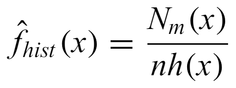
The choice of bin width is the most important decision when creating a histogram. There are many different choices for binwidth.
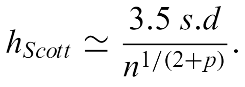
is used when the population resembles a normal distribution, where ⅓ is replaced by 1/(2 + p) for multivariate datasets with p dimensions. The MSE has a bias that shrinks with shrinking h and a variance that decreases for increasing h. Other choices of bin width work to balance the tension between the two.
Histograms have several problems:
Even though there are all these drawbacks, histograms are appropriate when the original data is binned
Convolve discrete data with a kernel to create a smooth density. However, there are many possible choices for the functional form and smoothing parameter/bandwidth for the kernel.
A constant bandwidth kernel estimator for i.i.d. random variables has the form
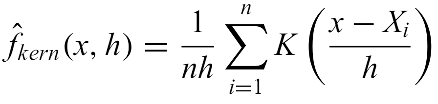
where K is the normalized kernel function.
Mean integrated square error - criterion for applicability of a KDE to an underlying pdf.
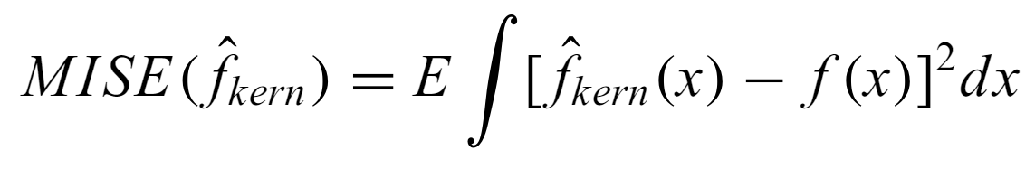
where E is the mean. It is also the sum of bias and variance terms, so the optimal bandwidth is chosen to minimize the MISE.
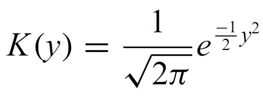
the Gaussian density with mean 0 and variance 1 is a very common choice of kernel, though it is not optimal for minimizing MISE. Other choices include the
Epanechikov kernel - an inverted parabola kernel over -1 to 1
and an inverted triangle. The boxcar kernel is a rectangle, though it has weaker performance.
Finding the correct bandwidth is very important to minimizing the MISE, and there are many difference possible choices.
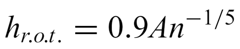
where A is the minimum of the standard deviation and interquartile range is a rule of thumb bandwidth, though it doesn't work for multimodal distributions.
It is, in general, very difficult to minimize the MISE by direct calculation. A way around this is with
Cross-validation - jackknife the dataset and calculate the KDE for each one. The average loglikelihood over these datasets is
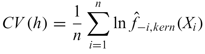
and the optimal bandwidth maximizes CV. There is a least-squares version that is resistant to outliers.
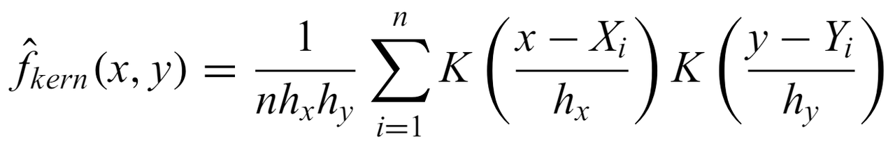
In multiple dimensions, the estimator can be a single multivariate density function or the product of univariate kernels.
There are oftentimes datasets with multiple peaks or detailed structure over a range of scales. In this case, the previous KDEs lose underlying information.
There are multiple different approaches one can use. For example, a particularly simple one is
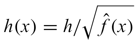
where h is the global optimal bandwidth and f is an approximation of the pdf.
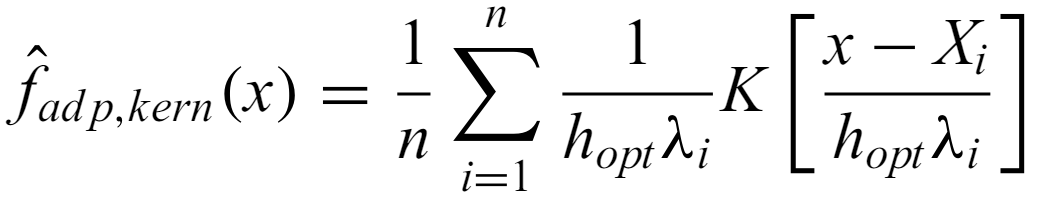
A more complicated but widely applicable approach starts with a first estimate of the density f~ using a standard kernel and the optimal constant bandwidth. Then, λ, the local bandwidth factor is obtained at each x point
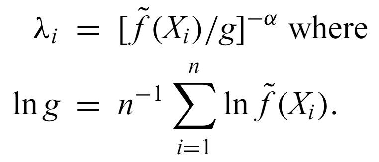
where g is the geometric mean of the first estimator and α is a sensitivity parameter between 0 and 1 (how sensitive the final kernel is to local variations). Then, finally, the adaptive estimator at x is given by
k-th nearest neighbor - Exactly what it sounds like. The density estimator based on it is given by
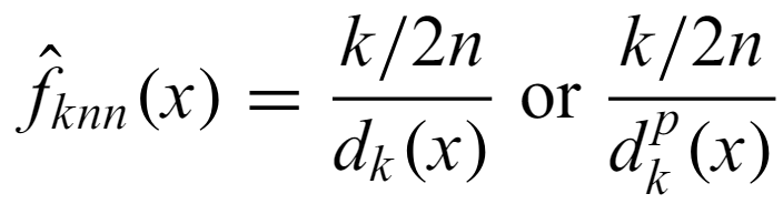
where p is the dimensionality. It is useful in datamining, but it has disadvantages: it is not a pdf (not normalized), it is discontinuous, prone to local noise, no general best choice of k.
Many datasets are multivariate tables of properties. Many scientific questions are about quantifying the dependence of a response variable (dependent variable) y on one or more independent variables x. Here we look at methods that do not guess the true parametric functional relationship. It should be used when the physical processes linking y and x are not known. These are not common in astronomy, but should be moreso.
NW estimator - For i.i.d. bivariate data, the estimated regression function given by
It is a weighted local average of the dependent variable. Also the least-squares regression fit of y as a function of x when the y values are averaged over a window of width 2hx centered at Xi. This concept has been generalized to fit higher order polynomials in these windows to more accurately model gradients and can be generalized to multivariate problems, such as with the LOWESS method that involves calculating kernels for local polynomial regression.
Range - equivalent to local bandwidth
Spline smoothing - A chosen function (usually a cubic) is fitted locally to data with a roughness penalty to constrain the smoothness. The curve is evaluated at knots (usually between points) rather than data points themselves. Smoothing splines have small bias, but don't necessarily minimize MISE.
There are multivariate extensions to this type of regression, including
Kriging - Least-squares interpolation method for irregularly spaced data points (more on this later).
Here they give examples of histograms, quantile functions, and representing measurement errors. There are some examples of different kernel smoothers (both constant and adaptive) as well as how measurement errors impact these. They also show some examples of nonparametric regression like spline fits, NW estimators, local regression, and LOESS.
Fitting models to data is extremely common in astronomy. Could be a simple line or a complex model.
Involves estimating functional relationships between dependent and independent variables. with random error. For example, the expectation of the response variable Y given the independent variable(s) X is a function of X, where the function depends on the model parameters, plus noise. This is in general a multivariate problem, but this book focuses on bivariate regression (though the methods used are usually also applicable in higher dimensions). The goal of regression usually focuses on estimation of the parameters of the function and their confidence interavls. The independent variable is assumed to have no uncertainty, thought this is accounted fro with measurement error models.
Linear regression model -
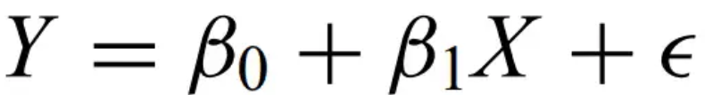
where X is the independent variable, Y is the dependent variable, beta contains the unknown intercept and slope.
Structural models - when the X's are random variables
Functional models - when the X's are deterministic.
Intrinsic scatter - exactly what it sounds like. Occurs when Y values do not fall exactly on the parametric curve. These are intrinsic errors in the response variable. When the Y values should lie precisely on the curve, the scatter is measurement error.
So far, we assumed X and Y are RVs that take on real values. However, many astronomical situations use regression on different data structures. X could be location in an image, or wavelength in a spectrum, or other fixed variables with predetermined locations.
Poisson regression - the above situation and when Y is an integer variable with small values based on a counting process. (more on this later)
Logistic regression - When Y is a binary variable with values of 0 or 1 (or a multivariate categorical variable) (more on this later)
Ordinary regression should only be used when the scientific problem naturally specifies a dependent variable. In statistics, “linear models” refer to any model that is linear in the parameters, not the model variables. This is opposed to just a straight line, per se.
Mixtures - sums of linear models. They are also linear themselves.
Once a model is chosen, can use any of these previously described parameter estimation techniques.
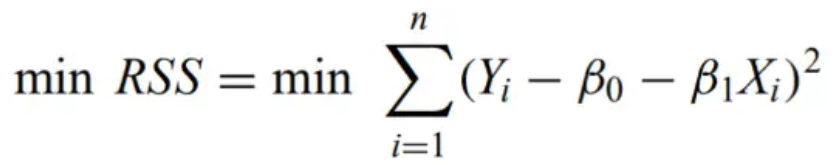
Residual sum of squares - The sum of the squares of the observed value minus the model predictions.
Ordinary least-squares estimator - the estimator for the linear regression model that minimizes the RSS:
The estimates of beta are given below
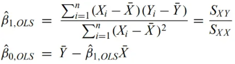
where SXY represents the sum of squared residuals of X and Y.
The estimator of the variance is RSS/(n - 2). These are also the MLE
Standard error - The sample standard deviation divided by SXX
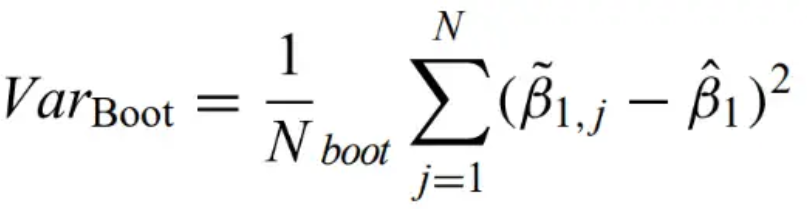
It is oftentimes best to use bootstrap to determine uncertainties.
Paired bootrap - A random sample (X1,Y1), (X2,Y2),… ,is drawn from two populations (X1,Y1), (X2,Y2),… with replacement. The estimators are generated for each bootstrap (the same way as the equations above), and the variance is average sum of square residuals between the estimator and the bootstrapped estimator.
Classical bootstrap - Applied where resamples are obtained by random selection of the residuals from the original model fit, rather than by random selection from the original data points.
M-estimation - and example of a robust estimator that keeps all points but minimizes a function with less dependence on outlying points. For any function psi and any solution beta,
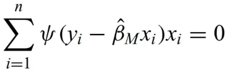
is an M-estimator. MLE and least squares are both examples of M-estimators.Asymptotically consistent, unbiased, and normally distributed. Classical least squares when psi equals x, but this is not robust to outliers. Some more robust examples follow.
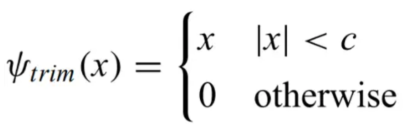
Trimmed estimator - trims outliers with large residuals
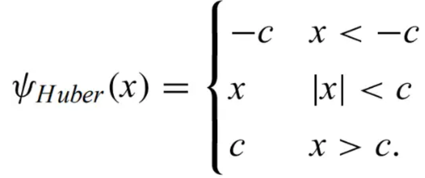
Huber estimator - keeps all points but sets points with large residuals to a chosen value. The optimal value is 1.345 for normal distributions.
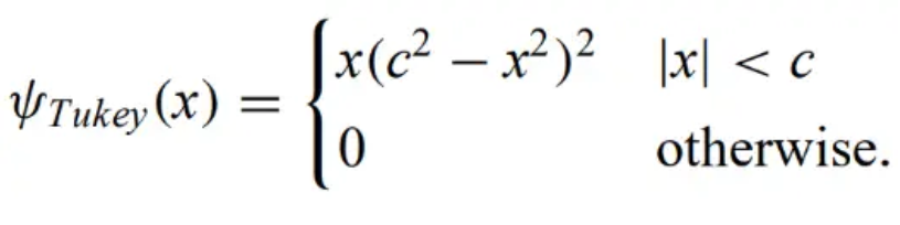
Tukey's bisquare/biweight function - trims very large outliers and downweights intermediate outliers. For this reason, it is a redescending M-estimator.
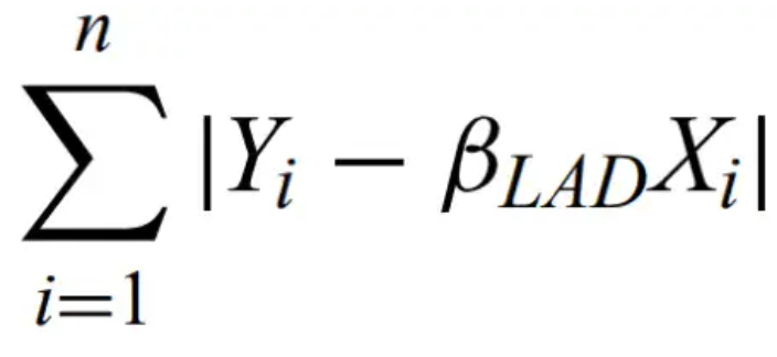
Least absolute deviation estimator - minimizes
Least trimmed squares estimator - minimizes

where q = (n + p + 1)/2, and p is the number of parameters. LTS is very robust.
Thiel-Sen median slope - find the median of the n(n+1)/2 slopes of lines defined by all pairs of data points.
It is common to get uncertainty measurements on each individual data point. This changes regression.
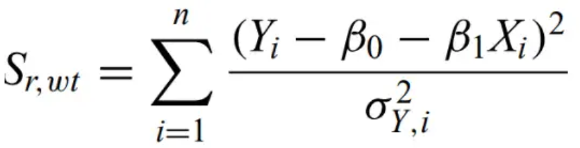
Minimum χ2 regression - a weighted least-squares regression procedure, requires minimizing
Pearson's χ2 test - given the null hypothesis that the data are drawn from a population following a given model, the probability that the χ2 statistic for n observations exceeds a chosen value is asymptotically equal to the probability that a χ2 random variable with k-p-1 degrees of freedom exceeds x. Created originally for the multinomial experiment.
There is often very well-defined uncertainties on both X and Y.
Measurement error/errors-in-variables/latent variable models - Regression models that use a hierarchical structure to allow for both known and unknown measurement errors.
Latent - variables in the regression equation
Manifest - variables X and Y in the measurement equations.
These types of models are very flexible.
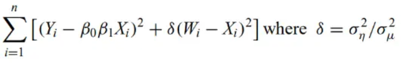
Orthogonal distance regression - algorithm to minimize the squared sum of distances for data with constant error, available for both linear and nonlinear functions.
Simulation-extrapolation (SIMEX) algorithm - Monte Carlo procedure to reduce least-squares regression biases arising from measurement errors.It simulates datasets based on the observations with a range of artificially increased measurement errors.The parameter of interest is estimated for each simulation. Plot the estimated parameter versus the total measurement error. The resulting curve is extrapolated to zero measurement error.
Maximum likelihood procedures are in general more flexible than least-squares for regression, though they are more difficult to use.
One common method for regression is least-squares estimation that minimizes the residual sum of squares with respect to the vector of parameters.
Poisson regression - when response variable is a result of a Poisson process. Events are assumed independent. Takes advantage of nonnegativity and integer nature.
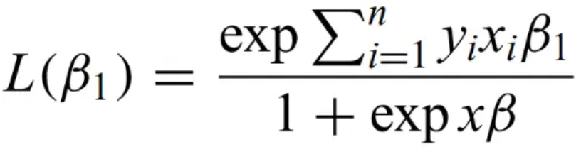
Logistic regression - when response variable is binary. Assumes that the logit is a linear function of the independent variables:
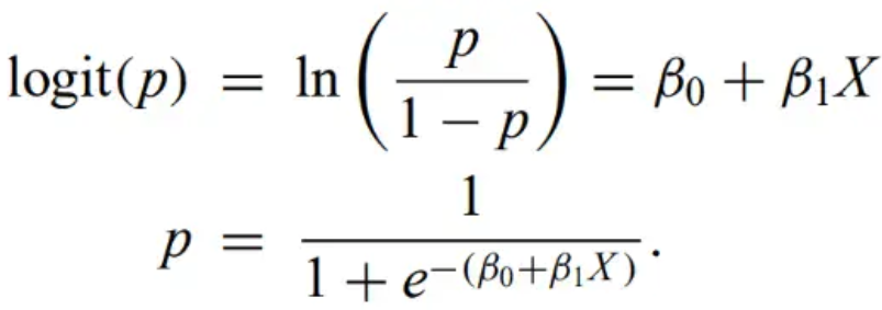
Regression coefficients can be obtained by MLE, maximizing
Getting best-fit parameters does not guarantee that the model actually fits the data. Most of the time, fits are not unique.
Coefficient of determination - A good model should account for most of the scatter in the original data. This is quantified in the R2 statistic,
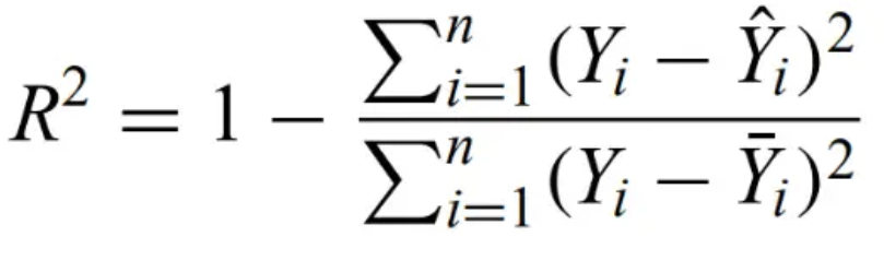
, the ratio of the error sum of squares to the total sum of squares. A successful model has R2 approach 1.
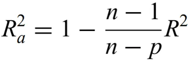
Adjusted R2 - penalizes number of parameters
Cross-validation - a portion of the dataset is withheld and used to evaluate the regressed model. When CV is repeated more and more times, it approaches jackknifing.
Most astronomers don't think very hard about the choices they make during regression, but they should.
This chapter has many examples. There is linear regression with heteroscedastic measurement errors, linear modeling using ordinary and weighted least squares, generalized linear modeling using glm, robust regression using robust M-estimators and Thiel-Sen, and linear and non-linear quantile regression.
Multivariate data is very common in astronomy (e.g. data tables)
The goals of multivariate analysis are to:
Covariance matrix - measures how variables vary with each other.
There are many different choices for defining distances between datapoints in p space. When all the units are the same, the natural metric is the
Euclidean distance - flat space distance
Minkowski metric - generalization of Euclidean distance for different m values
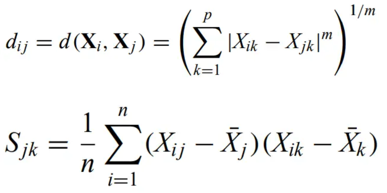
m = 1 is the Manhattan distance - distance measured only along grid lines. m = 2 is Euclidean, and m going to infinity gives the maximum or Chebyshev distance.
Can use weighted distances if measurement errors are known.
Distance matrix - matrix with all the distances between each element.
In astronomy, this is difficult because the variables do not have the same units. An easy solution is to standardize all variables by offsetting each to zero mean and unit standard deviation and then use euclidean distance.
Multivariate normal distribution - the natural extension of the normal distribution
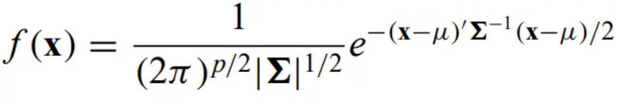
mu is the population mean, sigma is the population covariance matrix (', -1, || represent transpose, inverse, and determinant, respectively).
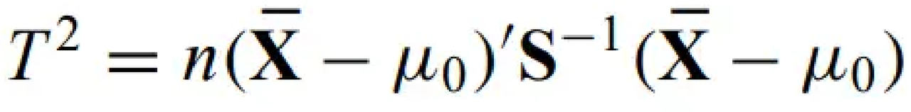
Hotelling T2 - multivariate generalization of student's t
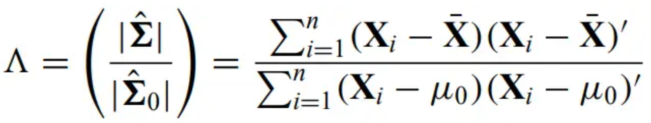
Wilks' lambda - generalization of likelihood ratio test
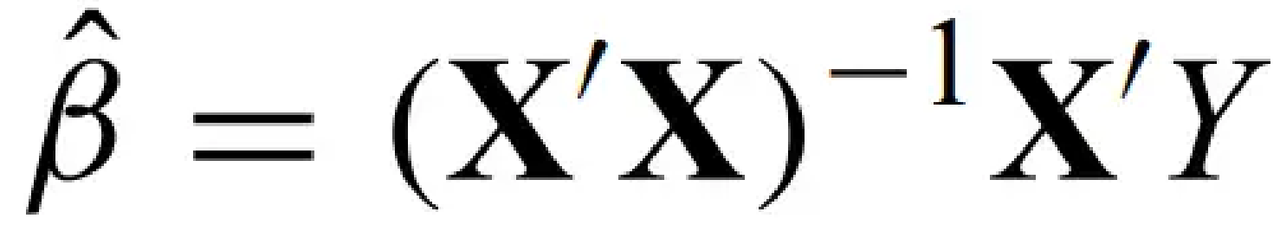
It is straightforward to extend linear regression to multivariate data, assuming only one response variable. Just replace X by a matrix and beta with a vector.
The extension of the least-squares estimator for the regression coefficients is
Ill-conditioning - Linear regression is unstable when variables are colinear
Least absolute shrinkage and selection operation/lasso - least squares regression model based on robust constraints.
Principal components analysis - models covariance structure with linear combinations of the variables. Finds linear relationships that account for the most variance in the data. It simultaneously studies linear relationships between properties and reduces dimensionality.
First center the data, then make covariance matrix, find evals and evecs of covariance matrix (these are variances and PCA components, respectively), plot each data point in PCA space. Classify data by looking for clusters or make images of each PCA component, then finally determine the physical meaning of the PCA vectors.
Independent component analysis - Assume that the underlying sources are independent. want to maximize negentropy. Use PCA to reduce dimensionality, then find the independent components. They are uncorrelated, but not perpendicular. However, they are independent.
Bivariate histograms, scatter plots, and contour plots are common in astronomy. One can also use a matrix of univariate or bivariate plots
R has some different ways of visualizing higher-dim data, but we never really went over this section in class.
There are examples in the book of univariate tests of normality and boxplots and Q-Q plots. They give a tutorial on how to prepare a multivariate dataset for analysis. They demonstrate bivariate relationships with a pair plot. There is an example of PCA as well, along with multiple regression and MARS nonlinear regression. There are also some techniques of multivariate visualization techniques on display.
Subpopulations show up all the time in multivariate data
Astronomers are always classifying things into different groups and classes based on various properties. However, most of the old classifications were subjective. There are also objective and statistical ways of doing this, even if the human eye is very good at it naturally.
Assume all datasets consist of n objects with p properties, with members from k subpopulations.
Unsupervised clustering techniques - Used when the number, location, size, and/or mophologies of the groupings are unknown. They look for groupings based on proximity using some distance measure in p-space. Results are uncertain and depend on distance measure.
Supervised classification - the combination of using a training set to characterize the groupings in the dataset and establishing discrimination rules on the training set and applying them to a new test set.
classification/decision trees - fall into subgroups based on different ranges of multiple variables. a better definition later.
Normal mixture model - the dataset is assumed to consist of k multivariate Gaussians. MLE or Bayesian are used to obtain the number of groups and their mean and variance.
Data mining - methods of classifying objects in very large datasets
Machine learning - allow the system to improve its own performance as more data are treated. There are many methods, including both unsupervised and supervised classification using decision trees, neural networks, support vector machines, and Bayesian networks.
Center - necessary for many clustering and classification algorithms. The natural choice is the centroid, but the median is more robust, so use medoids.
It is important to be able to measure the success of any given procedure. The probability of misclassification can be combined with asymmetries as the cost of misclassification. A big question in science is how to balance the cost. For example, if the sample is very large, it would be more costly to waste time on erroneous measurements, but if the sample is small, it might be more costly to lose possible targets.
Expected cost of misclassification - exactly what it sounds like

Hierarchical clustering methods - find groupings without parametric assumptions or prior knowledge. It beings with each point in its own cluster. The clusters that are closest together are merged. This is repeated n-1 times until the entire dataset is within a single cluster.
Tree/dendrogram - The result of hierarchical clustering. It shows every step of the process and describes how and when each cluster merged.
HC is very sensitive to the distance metric chosen. There are a few common choices:
Single linkage/friends-of-friends/nearest-neighbor clustering - the distance metric is the distance to the closest cluster member. Tends to produce unphysical elongated clusters.
Minimal spanning tree - subset of edges on a graph that connect all points with the minimum total weight (usu. distance)
Complete linkage - distance to the furthest cluster member is the metric
Average linkage - intermediate choice where the distance metric is the average distance to cluster members
Ward's minimum variance - Clusters are merged to minimize the increase the sum of intra-cluster summed squared distances.
k-means partitioning - start with k seed locations that represent the cluster centroids and iteratively reassign each object to the nearest cluster to reduce the sum of within-cluster squared distances. Usually converges rapidly. Choices that must be made: number of clusters k, initial seed locations (can have some impact), and must define the centroid. Choosing mean is sensitive to outliers, so sometimes use k-medoid partitioning. Careful that the summed distances, not squared distances, are minimized.
Previous methods assume all objects belong to a cluster, but, in astronomy especially, this is not always the case, such as background stars.
Bump hunting - start with the full dataset, progressively shrink a box with sides parallel to the axes. The box face is contracted along the face that most increases the mean density or statistic. After the peak location is located, the box may be expanded if density increases. Repeat to find other bumps.
DBSCAN (the best) - requires a minimum number of points within a specified reach distance. A cluster around an object with at least the minimum number of points within the reach expands naturally to include all density-reachable points. This continues until the criteria are broken. Unclassified points are considered noise.
There are other similar methods such as OPTICS, BIRCH, DENCLUE, CHAMELEON, etc.
Distinction between white noise and peaked distributions is bump hunting and distinction between one or more peaks is a test for multimodality.
Mixture models - Data are assumed to consist of some number of a given model form. Normal mixture models assume data are in k ellipsoidal clusters with MVN distributions.
There is a probabilistic method to assigning objects to more than one cluster (soft v. hard).
The most common model for supervised classification is MVN distribution.
Linear discriminant analysis - LDA for two classes is geometrically the same as projecting p-dim data point cloud onto a 1D line in p-space that maximally separates the classes. Separation is measured by the ratio of between-cluster variance B to the within-cluster variance W. Maximum separation occurs for

LDA is similar to PCA but has a different purpose. PCA finds linear combinations of variables that explain the most variance for the whole sample, and LDA finds linear combinations that separate classes within the sample. LDA vector a is obtained from a training set before being applied to new data.
Support Vector Machines - class of generalized LDAs. Dataset mapped by nonlinear functions onto a higher dimensional space so that classes in the training set can be separated using linear discrimination.
Classification trees - dividing a multivariate training sample into classes by progressive splitting
k-nearest-neighbor/memory-based classifier - related to nearest-neighbor and local regression density estimation techniques. Cluster membership is determined by the memberships of the k nearest-neighboring points in the training set. DANN is analogous to DBSCAN.
Automated neural networks - provide an environment where LDs are obtained in a space that has been nonlinearly mapped to from the original variables. weights learned from the training set. Basically, they use nonlinear rules to find classes.
There are many good examples in this chapter. Including unsupervised clustering using hierarchical clustering and dendrograms, DBSCAN, mixture models, and model based clustering. There is also supervised classification using LDA, k-nn, and single layer neural networks. There are examples of CART and SVM.
Astronomy is an unusual scientific discipline because there are a lot of upper limits on data points, and truncation by sensitivity limits is very common.
Censoring - object is known to exist but the object is undetected in the desired property. Can be left-censored (upper limits) or right-censored (lower limits)
Random left-censoring - some extraneous factor causes objects to be undetected (like poor sky conditions on a telescope)
Truncation - undetected objects are completely missing from the dataset.
Survival function - the probability that an object has a value above some specified level

Hazard rate - the derivative of the survival function. Also, the pdf divided by the survival function.

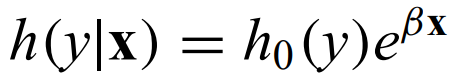
Proportional hazard model - A hazard function with an exponential decay h(x) = h0e-βx.
Cox regression - estimation of the β dependencies
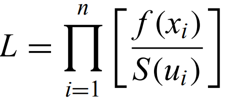
If the distribution is known already, ML methods can be used, even with censoring and truncation. The likelihood is given by the following

Once L is established, all of the tools from chapter 3 are applicable. There are some special cases given in the book where the solutions are particularly easy.
Nonparametric estimation of censored CDFs are straightforward generalizations of the edf.
When left-censored, the cumulative hazard function is

where d is the number of objects at value xi (1 without ties).
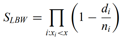
Kaplan-Meier estimator - Does not change values at censored data. with left-censored data, the size of the jumps grows at lower values as the number of remaining objects becomes small

Can obtain the KM estimator by a redistribute algorithm, where the weight of each upper limit is redistributed equally among the lower detections.
Can use two sample tests to ask “what is the probability that two censored datasets do not come from the same distribution.” Generally the same as classical nonparametric two-sample tests but with weights (scores) assigned to censored data.
Gehan test - generalized Wilcoxon test


General statistic for testing the null hypothesis that the k hazard rates are the same

where y is the number of objects at risk (not yet detected), d is the number of ties in the jth sample at value xi. N is total number of objects, j denotes individual samples. There are many common choices for the weights W.
Logrank test - W = yi, the number of objects not yet detected. Equals the sum of the failures observed minus the conditional failures expected computed at each failure time (the difference between observed and expected failures in one of the groups).
Gehan's test - W = yi2
Peto-Peto test - W = yi times the KM estimator.
Fleming-Harrington tests - use various functions of the KM estimator as weights.
logrank is more powerful than generalized Wilcoxon when proportional hazard applies, while generalized Wilcoxon are more effective than logrank when sample differences are greater at the uncensored side of the distribution.
First use a hypothesis test for correlation like Spearman's rho or Kendall's tau. With censoring, the generalizations of Kendall's tau are preferred

nc is the number of concordant pairs (with positive slope in x,y). nc is number of disconcordant pairs (with negative slopes). nt is the number of ties.
There are many methods for linear regression with censoring.
Accelerated failure-time model - and example of exponential regression, a standard linear regression model after a logarithmic transformation of the dependent variable. Helps with censored variable has a wide range of values (over orders of magnitude)

Proportional hazards model/Cox regression - mentioned before, has exponential hazard rate. For two objects with different covariate values, the hazard rates are proportional to each other as the ratio of the exponential parts.
Iterative least squares - familiar additive linear regression model is appropriate if the censored variable and covariates have similar ranges.
Buckley-James line estimator - variant to the MLE linear regression. permits non-gaussian residuals around the line. Trial regression is done, nonparametric KM estimator is computed and used as the distribution for the scatter. censored data points are moved downwards to new locations based on KM. likelihood maximized to obtain new estimates, and the procedure is iterated.
Akritas-Thiel-Sen - works well with doubly censored data or with bad outliers
No knowledge of how many undetected sources exist (flux limited surveys).
If the underlying distribution is known, then parametric analysis can proceed based on likelihood
where u are the tructation limits, f is the pdf, and S is the survival.
Lynden-Bell-Woodroofe estimator - nonparametric MLE for randomly truncated data. Unbiased, consistent, generalized MLE of underlying distribution
Here there are examples of the KM estimator, applying two-sample tests with censoring, multidimensional problems with censoring, and the LBW estimator for truncation.
Time-domain astronomy focuses on studying variable phenomena. However, much difficulty comes from the fact that a lot of astronomy nata is not evenly spaced in time and measurements often have heteroscedastic errors.
Procedures for evenly spaced data are well-known
Trend - when the average value of a time series changes with time. A global linear trend has the same form as linear regression, though X is the response and t is the independent variable, for times series analysis
Low-pass filter - smoothing to reduce variance from short-term variations
high-pass filter - examining residuals after fitting a regression model to reduce long-term trends
Differencing filter - commonly used to remove various types of trends (global, periodic, stochastic, etc.) to reveal short-term structure. One example is plotting the difference between consecutive points instead of the points themselves.
State-space model - mathematical model with input, output and state variables related by first-order ODEs or difference equations. can be constructed to fit simultaneously long-term ternds, periodicities, and short-term autocorrelation.
Autocorrelation - measure of correlated structure in a time series. Basically, how well a signal correlates with a delayed version of itself.
Autocorrelation function - quantifies how values at different separations (in time) vary together
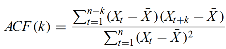
where k is the lag time and is an integer, the numerator is the sample autocovariance function, and the denominator is the sample variance. Strong ACF values for a given k imply autocorrelation on that time scale.
Correlogram - the plot of ACF(k) for a range of k values. Often have confidence intervals for the null hypothesis that no correlation is present.
White noise - random uncorrelated noise (usu. gaussian). It produces near-zero values in the ACF (ACF(0) = 1, trivially).
Long-term memory - What it sounds like. Time series with this property have non-zero ACF values for a wide range of k.
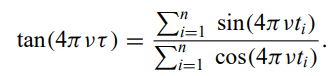
Periodic variations in the time series produce periodic variations in the ACF - natural application to use Fourier transform.
Residual time series - TS after trends have been removed. This is done because ACFs are difficult to interpret when trends and stochastic variations are both present.
Stationarity - temporal behavior that is unchanged by an arbitrary time shift.
The concept of an average is not relevant to nonstationary processes. A concept that is often applied to residuals after a model has been fitted.
Weakly stationary - functions with constant moments, like the mean and autocovariance but that change in other ways.
Nonstationarity - Opposite of stationarity, clearest examples are systems that change abruptly.
Change-point - The point in time when the variability characteristics abruptly change.
Spectral/Fourier analysis - the transformation of a signal from the time domain to the frequency domain. Signals from periodic phenomena are much more concentrated in frequency space.
Smoothing methods (Chapter 6) can very simply be applied to (evenly-spaced) time series data. One of the simplest methods is
Central moving average - calculates the moving average within a certain window, across the entire dataset.
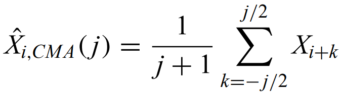
where the bandwidth is j time intervals. This can be modified to use median instead of mean, using only past values, weighting each value, etc.
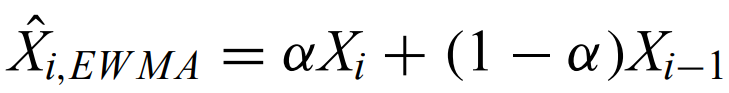
Exponentially weighted moving average - used for time series with short-term autocorrelation. It is called as such because the current value is a weighted average of all previous values with weights decreasing exponentially with time.
Variance is increased when autocorrelation is present. This can be thought of as a decrease in the number of independent measurements because the process is periodic.
Partial autocorrelation function - Gives autocorrelation while removing the effects of correlations at shorter lags. The value of PACF(p) is found by successively fitting autoregressive models with order 1,2,…,p and setting the last coefficient of each model to the PACF parameter. For example, AR(2) has

Lag k scatter plot - plot all x(t) against x(t+k). Random scatter implies uncorrelated noise and linear relationship points toward stochastic AR behavior. Circular distribution suggests a periodic signal, and clusters of points suggest nonstationary time series with classes of variable behavior.
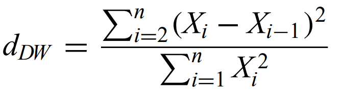
Durbin-Watson statistic - a simple measure of autocorrelation in evenly spaced time series. Value of 2 means no AC, higher is positive, lower is negative.
Random walk - the simplest stochastic autocorrelated model, where each step is the previous plus a guassian white noise term. Starts with an ACF of 1 that decreases with increasing k.
Autoregressive model - Generalization of the random walk that permits dependencies on more than just the previous step (with different weights). Has ACF(k) = the first constant to the kth power.
Moving average model - current value depends on past values of the noise rather than the variable itself.
ARMA(p,q) model - A combination of AR and MA models.

Autoregressive integrated moving average model - combines ARMA and random walk, since ARMA is stationary.
Volatility - another word for heteroscedasticity.
(Generalized) Autoregressive conditional heteroscedastic model - variance is assumed to be a stochastic autoregressive process depending on previous values.
Occurs frequently in astronomy.
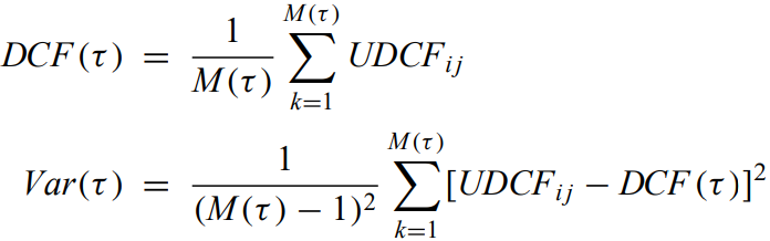
Unbinned discrete correlation function - computes autocorrelation function in a way that avoids interpolating unevenly spaced data on a regular grid.
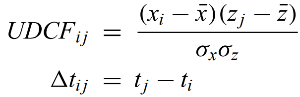
where x and z are datasets and t is the time.
Discrete correlation function - average of the UDCF
Structure function - measure of autocorrelation. average over the time series of the difference between x(t) and x(t+tau) to the qth power.
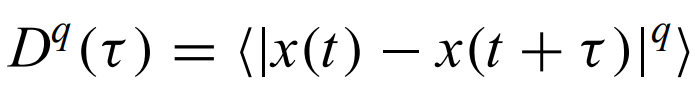
when q = 2, this is known as the variogram - alternative to ACF (more on this next chapter)
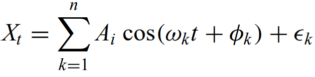
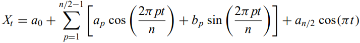
In Fourier analysis, a time series that is dominated by sinusoidal patterns can readily be modeled as
Power spectrum - the fourier transform of the autocovariance function
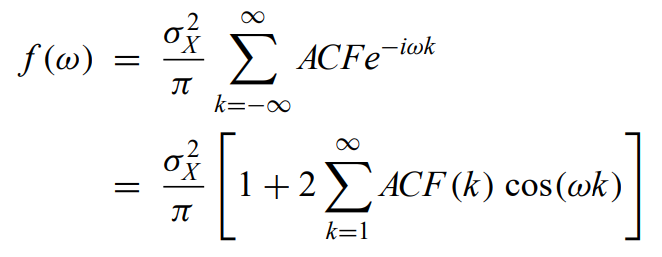
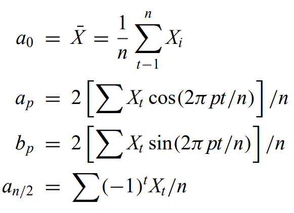
Spectral analysis - power spectrum usually must be estimated from the time series measurements of evenly spaced data. Usually with the finite fourier series
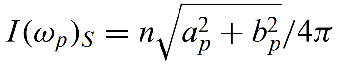
Periodogram - a histogram of the quantity I(omega) against omega
The periodogram has limitations: high noise, biased, unreasonable assumptions (infinitely long and evenly spaced data with stationary sinusoidal signals)
Spectral leakage - power going into nearby frequencies when the time series is short compared to the period.
Can smooth to reduce variance in either the frequency or time domains.
Occurs more in astronomy than many other fields.
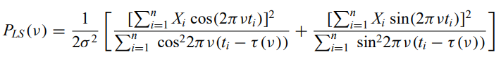
Lomb-Scargle periodogram - generalization of the periodogram for unevenly spaced data. Can be either a modified Fourier analysis or a least-squares regression to sine waves
Minimum string length - The sum of the length of lines connecting values of the time series as the phase runs from 0 to 2pi. For an incorrect period, the signal is scattered in phase and the string length is large.
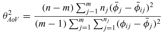
Analysis of variance (ANOVA) statistic - ratio of the sum of inter-bin variances to the sum of intra-bin variances
Significance levels are in general difficult to determine for periodigrams of unevenly spaced data, but for the LSP, the probability that some spectral peak is higher than z0 is:
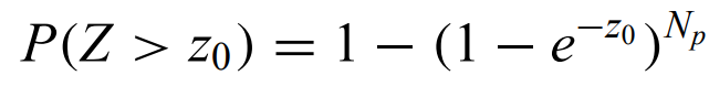
where Np is the number of independent periods. Widely used, but it has its problems. Assumes that there is a single periodic signal in white noise and that the variance is known in advance.
Nonstationary Poisson processes - Poisson process with underlying periodic variability. There are some periodograms that can be used in this case.
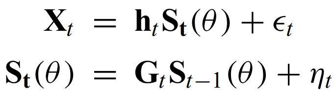
X is a vector of observed values for a collection of variables. S is the state vector that depends on the parameters theta, h is the matrix that maps the true state space into the observed space. G is the transition matrix that defines how the system changes in time. Epsilon and η terms terms are normal errors.
There are many ways to analyze nonstationary time series:
Regression for deterministic behavior - best-fit parameters can be estimated by least-squares, MLE, or Bayesian using standard regression or state space approaches.
Bayesian blocks and bump hunting - semi-parametric regression to characterize signals and detect change-points. Data is a sequence of events. Construct a likelihood assuming a sequence of constant flux levels with jumps at a number of change-points.
Change-point analysis - If likelihood methods establish the model of the initial state, the likelihood ratio test can find changes in the mean, variance, trend, autocorrelation, and other model characteristics. Nonparametric tests are often used to find structural changes.
Wavelet analysis - Wavelets transform time data to frequency space like fourier, but it is well-suited to nonstationary processes, especially if variations occur on a range of temporal scales. The transform is given by
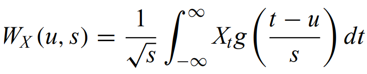
where Xt is the function being transformed, s is the scale, u is the time, and g is a simple basis function that falls rapidly to 0, like a gaussian. This process maximizes the temporal resolution at all frequencies by changing the area of each bin in frequency space (higher frequencies get better time resolution and worse frequency resolution and vice versa).
Singular spectrum analysis - PCA for temporal data, used for smoothing complex time series.
1/f/flicker/red noise or long-memory process - when variance increases with the characteristic time-scale and the power spectrum can be fit by a power-law at low frequencies. It is called 1/f because there is an inverse correlation of power and frequency in the Fourier power spectrum.
Short-memory - processes that can be understood with low-order ARMA models.
Long-memory processes can arise from a combination of many short-memory processes like the sound of a babbling brook. or from starspots, etc. Often modeled as an autocorrelation function that decays as a power law at large time lags.
Multiple variables might depend on each other in time.
Cross-correlation function - the second-order moments for a bivariate stochastic process are the two individual ACFs and the CCF:
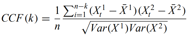
If the CCF shows a single strong peak at some lag k, this may reflect similar structure in the two time series with a delay. CCF can be generalized to multivariate using correlation matrix.
This approach is really uncommon in astronomy, so it is not discussed further.
Here there are examples of histograms, raw and smoothed time series, raw and smoothed periodograms, autocorrelation functions, autoregressive modeling, depictions of long-range memory, and wavelet analysis.
Spatial data is used all the time in photometry, though the third dimension is usually much less well defined. In addition, spatial point processes are applicable to much astronomical data in low dimensions.
Point processes - sets of irregular patterns in (usually) 2 or 3D space. Stationary if invariant under spatial translation. Isotropic if invariant under rotation
Intensity - λ, and
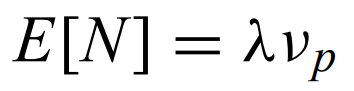
is the expected number of points in a unit of volume v. Follows a Poisson distribution for Poisson processes
Complete spatial randomness - a stationary Poisson point process where λ is constant across the space. Sprinkling sand grains on a table or background radiation in a detector.
Inhomogeneous - when λ varies with location.
Marked point processes - PP when there are associated nonspatial variables.
Spatial point process analysis usually begins with testing the hypothesis that the distribution is consistent with CSR. One thing that is often compared with CSR is the edf of the
Nearest-neighbor distribution -
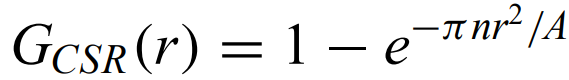
where A is the 2D area containing n points. Simulations are needed to account for edge effects and for small-n samples.
Some CSR tests are based on sums of nearest-neighbor distances
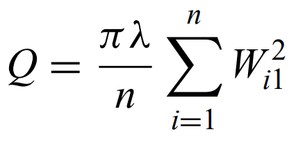
where lambda is average surface density of points and W is the Euclidean distance between i-th point and its nearest neighbor.
A modified Pollard's P performs well using the five nearest neighbors
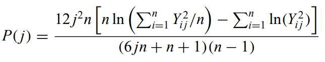
where j = 1 to 5 and Yij are distances between i randomly placed locations and the jth nearest neighbor.
Bias from edge effects is a big issue.
The unbiased MLE for the intensity of a stationary Poisson point process is the intuitive value: the number of points in a unit p-dim volume.
Moran's I and Geary's contiguity ratio c - Indices of spatial autocorrelation that are extensions of Pearson's coefficients of bivariate correlation. They detect departures from spatial randomness. Usually inverse distance weighted. For data grouped into m identical spatial bins
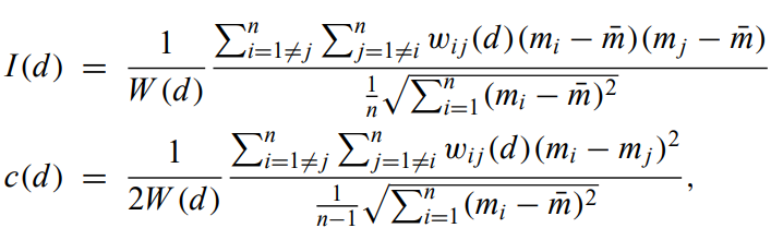
where mj is the count of objects in the jth bin. w is the matrix of the kernel function and W is the sum of w elements.
Correlograms - plots of I against d.
E[I] = -1/(n-1), E(c) = 1 for normal noise without clusters or autocorrelation. With strong autocorrelation, both approach 0
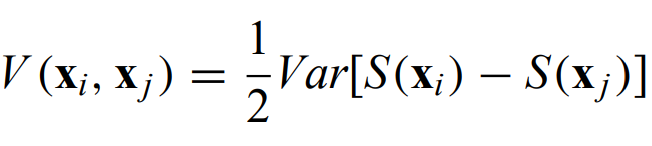
Variogram/semi-variogram - used to map the variance on different scales across the survey area. half the average squared difference between pairs of values is plotted against the separation distance.
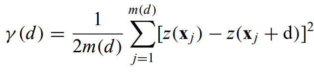
where m(d) is represents all of the pairs of points which are a distance d away from each other.
The variogram describes the second-moment properties of a spatial process S
For a stationary, isotropic, Gaussian spatial process, the variogram simplifies to
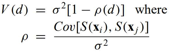
where rho is the spatial covariance function, d is the distance between data points at xi and xj.
Nugget effect - the σ2 offset at zero distance in a variogram. It is because of variations smaller than the minimum separation of measured points.
Sill - the rise to a constant value.
Range - the distance to the sill.
Variograms are usually modeled by simple functions (circular, parabolic, exponential, gaussian, power-law models exist)
There are local indicators of spatial association such as local Moran's I - averages the spatial variance among the k-nearest neighbors of the ith point.
If a SPP is a representation of an underlying continuous distribution, the interpolation is an effective way of estimating the distribution. Could either interpolate just density of points, but usually you interpolate some mark variable.
Because many things are influenced by the objects closest to them, it makes sense to use
Inverse distance weighted interpolation - exactly what it sounds like, the weighting scales inversely as a power law of the distance. The value z is calculated as
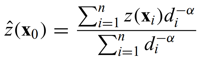
where d is the vectorial distance from the ith measurement to x0. α is chosen between 0 and 3, with smaller values giving smoother interpolations.
The most common method for interpolation of marked spatial data is
Kriging - a suite of related linear least-squares, minimum variance methods for density estimation in 2 or 3 spatial dimensions that localize inhomogeneous features instead of globally characterizing homogeneous distributions.
Ordinary kriging - want weightings at each point in the dataset to give the unbiased estimator of the continuous response variable z from measurements zi as
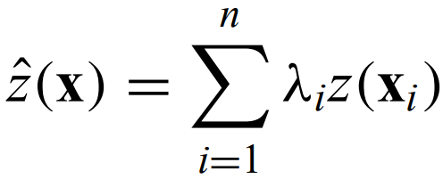
There are many types of kriging available: Simple kriging if the mean is already known, block kriging when the dataset is large and adjacent points can be merged, cokriging if two correlated variables are measured at each location, universal kriging first removes trends in the data, (external drift when a secondary variable can map those trends), nonlinear kriging when the trends are not linear in the variables, multitype kriging with categorical covariates, multivariate kriging with multiple interacting marked variables.
There are two very important global measures of clustering
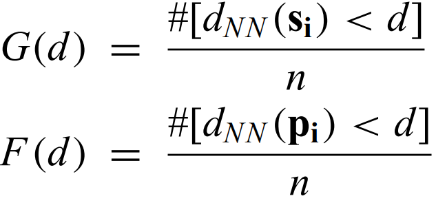
where these two functions are the cumulative distributions of the nearest-neighbor distances either from the data points (G) or from random locations (F)
Empty space function - F, above, because it is centered around empty locations.
F works better for weak clustering and G works better for strong clustering.
Ripley's K function - most widely used global measure of clustering. It is the average number of points within distance d of observed pointsdivided by the intensity.
Lieshout-Baddeley J function - (1-G)/(1-F), compares inter-event distances to distances from a fixed point.
Two-point correlation function - counts the number of objects in annuli (instead of circles) around each point. Measures the covariance of the nonuniform structure of the point distribution.
The parametric models for spatial analysis are similar to those for regression and time series. The hypothesis of CSR can be written as X = μ + epsilon, where epsilon is Poisson noise.This has no autocorrelation, clustering, or trend.
Geographically weighted regression - maps of several variables are available and you want to explain one map in terms of the others with a linear regression that takes spatial autocorrelation into account.
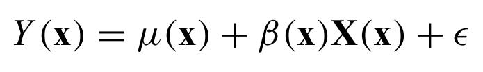
The response variable Y at location x depends on both the value of the covariates X and on neighboring values of Y, where epsilon is normal noise. The least-squares solution is found by minimizing
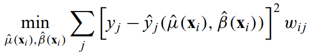
Spatial autoregressive model - assumes the regression coefficients are global, but the response variable is dependent on neighboring values. Can be written in a hierarchical fashion
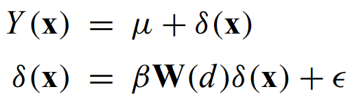
where mu is the mean, delta are the spatially correlated residuals, beta between -1 and 1 gives the strength of the spatial autocorrelation, epsilon is white noise, W is a normalized weight matrix that depends on the distance d from the data point x.
The p-dim distribution of neighbors provides more detailed information about local autocorrelation and clustering for point processes. Visualizations of these connections between nearby points are important to graph theory.
Delaunay triangulation - join all neighboring triplets of points with triangles.
Voronoi/Dirichlet/Thiessen tessellations - based on line bisectors perpendicular to the Delaunay line segments. Splits the space into polygons around the datapoint. Within a polygon, all points are closer to the associated data point (or set of data points, for higher orders) than any other (set of) point(s).
Pruning MSTs give a procedure to define a hierarchy of spatial clusters. discussed in chapter 9.
Useful in astronomy, since 2D sky positions are on a sphere.
Moments are not generally useful because of angles. Angular values must be summed vectorially. The average direction of a sample of angles is the solution of
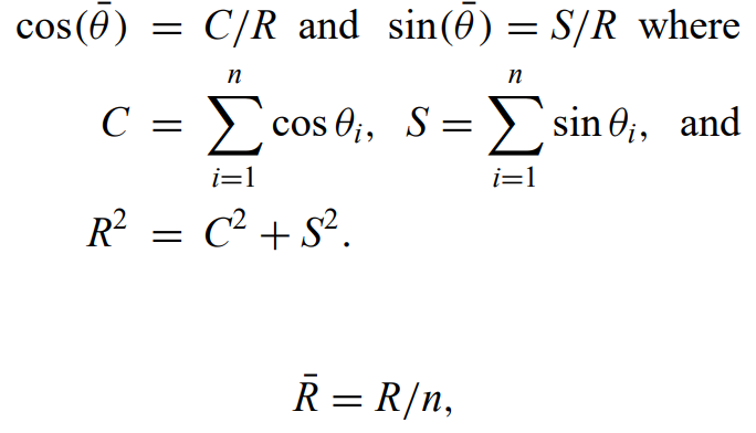
R/n is the mean resultant length, and it approaches 1 when the data are clustered towards one direction, and 0 when they are balanced.
Sample circular variance - 1 - Rbar.
Circular dispersion - a more useful measure of angular spread
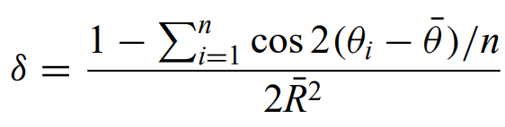
In this section there are 3D plots, characterization of autocorrelation with Moran's I and Geary's c, variogram analysis, characterization of clustering with K function, the two-point correlation function, examples of tessellations and applications to smoothing, spatial interpolation with IDW and ordinary kriging, discussion of spatial regression and modeling, and some examples of circular and spherical statistics.